pyxu_diffops.operator#
- class MfiDiffusion(dim_shape, extra_term=True, beta=1, clipping_value=1e-05, tame=True, sampling=1)[source]#
Bases:
_DiffusionMinimum Fisher Information (MFI) diffusion operator, featuring an inhomogeneous isotropic diffusion tensor. Inspired from minimally informative prior principles, it is popular in the plasma physics tomography community. The diffusivity decreases for increasing local intensity values, to preserve bright features.
The MFI diffusion tensor is defined, for the \(i\)-th pixel, as:
\[\begin{split}\big(\mathbf{D}(\mathbf{f})\big)_i = (g(\mathbf{f}))_i \;\mathbf{I} = \begin{pmatrix}(g(\mathbf{f}))_i & 0\\ 0 & (g(\mathbf{f}))_i\end{pmatrix},\end{split}\]where the diffusivity \(g\) is defined in two possible ways:
in the tame case as
\[(g(\mathbf{f}))_i = \frac{1}{1+\max\{\delta, f_i\}/\beta},\quad\delta\ll 1,\]
\(\quad\;\;\) where \(\beta\) is a contrast parameter,
in the untame case as
\[(g(\mathbf{f}))_i = \frac{1}{\max\{\delta, f_i\}},\quad\delta\ll 1,\]
The gradient of the operator reads
\[-\mathrm{div}(\mathbf{D}(\mathbf{f})\boldsymbol{\nabla}\mathbf{f})-\sum_{i=0}^{N_{tot}-1}\frac{\vert(\boldsymbol{\nabla}\mathbf{f})_i\vert^2}{(g(\mathbf{f}))_i^2}\;,\]where the sum is an optional balloon force
extra_term, which can be included or not.We recommend using the tame version, since it is better behaved: the untame version requires very small steps to be stable. Furthermore, we recommend including the extra term, because in this case the potential \(\phi\) can be defined.
- Parameters:
dim_shape (
NDArrayShape) – Shape of the input array.extra_term (
bool) – Whether the extra term arising from the differentiation of the MFI functional should be included. Defaults toTrue(recommended). If set toFalse(linearized MFI), the MFI diffusion operator does not admit a potential and theapply()method is not defined.beta (
Real) – Contrast parameter, determines the magnitude above which image gradients are preserved. Defaults to 1.clipping_value (
Real) – Clipping value \(\delta\) in the expression of the MFI diffusivity. Defaults to 1e-5.tame (
bool) – Whether tame or untame version should be used. Defaults toTrue(tame, recommended).sampling (
Real,list[Real]) – Sampling step (i.e. distance between two consecutive elements of an array). Defaults to 1.
- Returns:
op – MFI diffusion operator.
- Return type:
- class PeronaMalikDiffusion(dim_shape, beta=1, pm_fct='exponential', sigma_gd=1, sampling=1)[source]#
Bases:
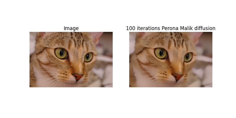
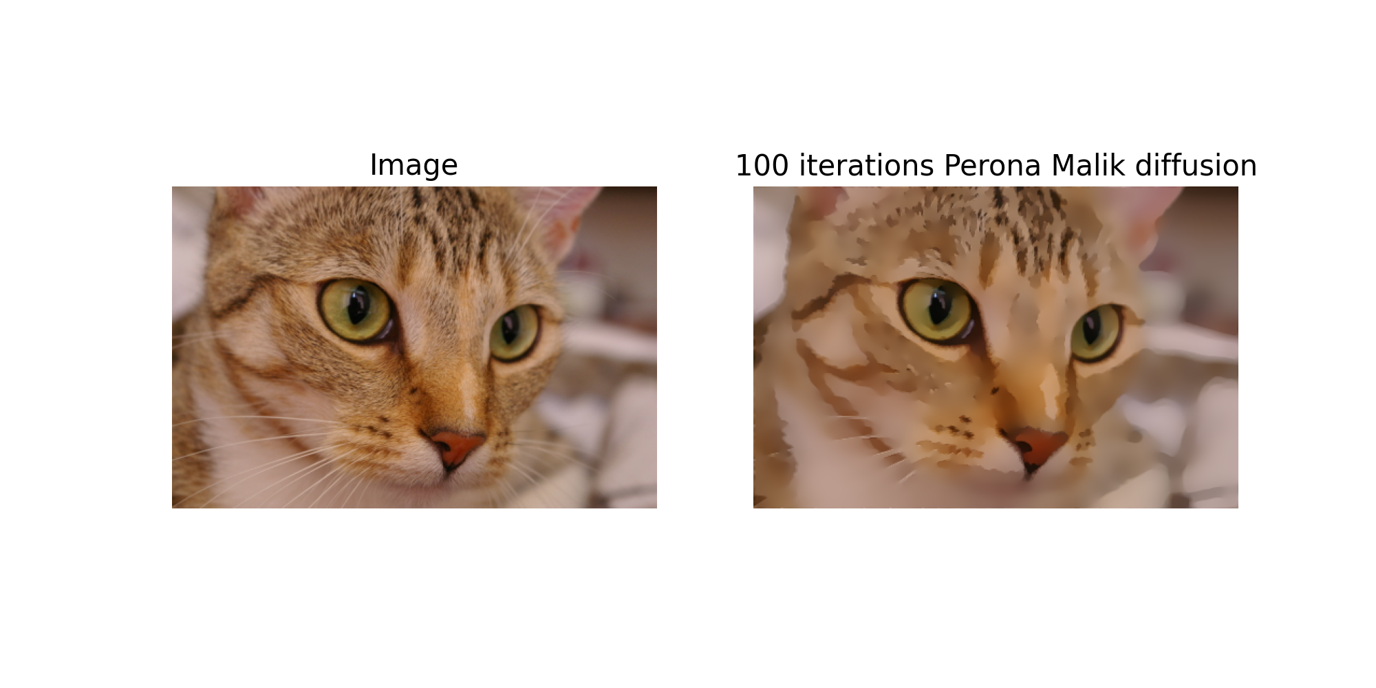
_DiffusionPerona-Malik diffusion operator, featuring an inhomogeneous isotropic diffusion tensor with Perona-Malik diffusivity. It can be used for edge-preserving smoothing. It reduces the diffusion intensity in locations characterised by large gradients, effectively achieving edge-preservation.
The gradient of the operator reads \(\nabla\phi(\mathbf{f})=-\mathrm{div}(\mathbf{D}(\mathbf{f})\boldsymbol{\nabla}\mathbf{f})\), where \(\phi\) is the potential.
The Perona-Malik diffusion tensor is defined, for the \(i\)-th pixel, as:
\[\begin{split}\big(\mathbf{D}(\mathbf{f})\big)_i = (g(\mathbf{f}))_i \;\mathbf{I} = \begin{pmatrix}(g(\mathbf{f}))_i & 0\\ 0 & (g(\mathbf{f}))_i\end{pmatrix},\end{split}\]where the diffusivity with contrast parameter \(\beta\) is defined as:
\((g(\mathbf{f}))_i = \exp(-\vert (\nabla_\sigma \mathbf{f})_i \vert ^2 / \beta^2)\) in the exponential case,
\((g(\mathbf{f}))_i = 1/\big( 1+\vert (\nabla_\sigma \mathbf{f})_i \vert ^2 / \beta^2\big)\) in the rational case.
Gaussian derivatives with width \(\sigma\) are used for the gradient as customary with the ill-posed Perona-Malik diffusion process.
In both cases, the corresponding divergence-based diffusion term admits a potential (see [Tschumperle] for the exponential case): the
apply()method is well-defined.- Parameters:
dim_shape (
NDArrayShape) – Shape of the input array.beta (
Real) – Contrast parameter, determines the magnitude above which image gradients are preserved. Defaults to 1.pm_fct (
str) – Perona-Malik diffusivity function. Must be either ‘exponential’ or ‘rational’.sigma_gd (
Real) – Standard deviation for kernel of Gaussian derivatives used for gradient computation. Defaults to 1.sampling (
Real,list[Real]) – Sampling step (i.e. distance between two consecutive elements of an array). Defaults to 1.
- Returns:
op – Perona-Malik diffusion operator.
- Return type:
Example
import numpy as np
import matplotlib.pyplot as plt
import pyxu.opt.solver as pysol
import pyxu.abc.solver as pysolver
import pyxu.opt.stop as pystop
import pyxu_diffops.operator as pyxop
import skimage as skim

# Import RGB image
image = skim.data.cat().astype(float)
print(image.shape)  # (300, 451, 3)

# Move color-stacking axis to front (needed for pyxu stacking convention)
image = np.moveaxis(image, 2, 0)
print(image.shape)  # (3, 300, 451)

# Instantiate diffusion operator
pm_diffop = pyxop.PeronaMalikDiffusion(dim_shape=(3, 300, 451), beta=5)

# Define PGD solver, with stopping criterion and starting point x0
stop_crit = pystop.MaxIter(n=100)

# Perform 50 gradient flow iterations starting from x0
PGD = pysol.PGD(f=pm_diffop, show_progress=False, verbosity=100)
PGD.fit(**dict(mode=pysolver.SolverMode.BLOCK, x0=image, stop_crit=stop_crit,
               tau=2 / pm_diffop.diff_lipschitz))
pm_smoothed_image = PGD.solution()

# Reshape images for plotting
image = np.moveaxis(image, 0, 2)
pm_smoothed_image = np.moveaxis(pm_smoothed_image, 0, 2)

# Plot
fig, ax = plt.subplots(1, 2, figsize=(10, 5))
ax[0].imshow(image.astype(int))
ax[0].set_title("Image", fontsize=15)
ax[0].axis('off')
ax[1].imshow(pm_smoothed_image.astype(int))
ax[1].set_title("100 iterations Perona Malik diffusion", fontsize=15)
ax[1].axis('off')
(
Source code,png,hires.png,pdf)
- class TikhonovDiffusion(dim_shape, sampling=1)[source]#
Bases:
_DiffusionTikhonov diffusion operator, featuring a homogeneous isotropic diffusion tensor with constant diffusivity. It achieves Gaussian smoothing, isotropically smoothing in all directions. The diffusion intensity is identical at all locations. Smoothing with this diffusion operator blurs the original image.
The gradient of the operator reads \(\nabla\phi(\mathbf{f})=-\mathrm{div}(\boldsymbol{\nabla}\mathbf{f})=-\boldsymbol{\Delta}\mathbf{f}\); it derives from the potential \(\phi=\Vert\boldsymbol{\nabla}\mathbf{f}\Vert_2^2\).
The Tikohnov diffusion tensor is defined, for the \(i\)-th pixel, as:
\[\begin{split}\big(\mathbf{D}(\mathbf{f})\big)_i = \mathbf{I} = \begin{pmatrix}1 & 0\\ 0 & 1\end{pmatrix}.\end{split}\]- Parameters:
dim_shape (
NDArrayShape) – Shape of the input array.sampling (
Real,list[Real]) – Sampling step (i.e. distance between two consecutive elements of an array). Defaults to 1.
- Returns:
op – Tikhonov diffusion operator.
- Return type:
Example
import numpy as np
import matplotlib.pyplot as plt
import pyxu.opt.solver as pysol
import pyxu.abc.solver as pysolver
import pyxu.opt.stop as pystop
import pyxu_diffops.operator as pyxop
import skimage as skim

# Import RGB image
image = skim.data.cat().astype(float)
print(image.shape)  # (300, 451, 3)

# Move color-stacking axis to front (needed for pyxu stacking convention)
image = np.moveaxis(image, 2, 0)
print(image.shape)  # (3, 300, 451)

# Instantiate diffusion operator
tikh_diffop = pyxop.TikhonovDiffusion(dim_shape=(3, 300, 451))

# Define PGD solver, with stopping criterion and starting point x0
stop_crit = pystop.MaxIter(n=100)

# Perform 50 gradient flow iterations starting from x0
PGD = pysol.PGD(f=tikh_diffop, show_progress=False, verbosity=100)
PGD.fit(**dict(mode=pysolver.SolverMode.BLOCK, x0=image, stop_crit=stop_crit,
               tau=2 / tikh_diffop.diff_lipschitz))
tikh_smoothed_image = PGD.solution()

# Reshape images for plotting.
image = np.moveaxis(image, 0, 2)
tikh_smoothed_image = np.moveaxis(tikh_smoothed_image, 0, 2)

# Plot
fig, ax = plt.subplots(1, 2, figsize=(10, 5))
ax[0].imshow(image.astype(int))
ax[0].set_title("Image", fontsize=15)
ax[0].axis('off')
ax[1].imshow(tikh_smoothed_image.astype(int))
ax[1].set_title("100 iterations Tikhonov smoothing", fontsize=15)
ax[1].axis('off')
(
Source code,png,hires.png,pdf)
- class TotalVariationDiffusion(dim_shape, beta=1, tame=True, sampling=1)[source]#
Bases:
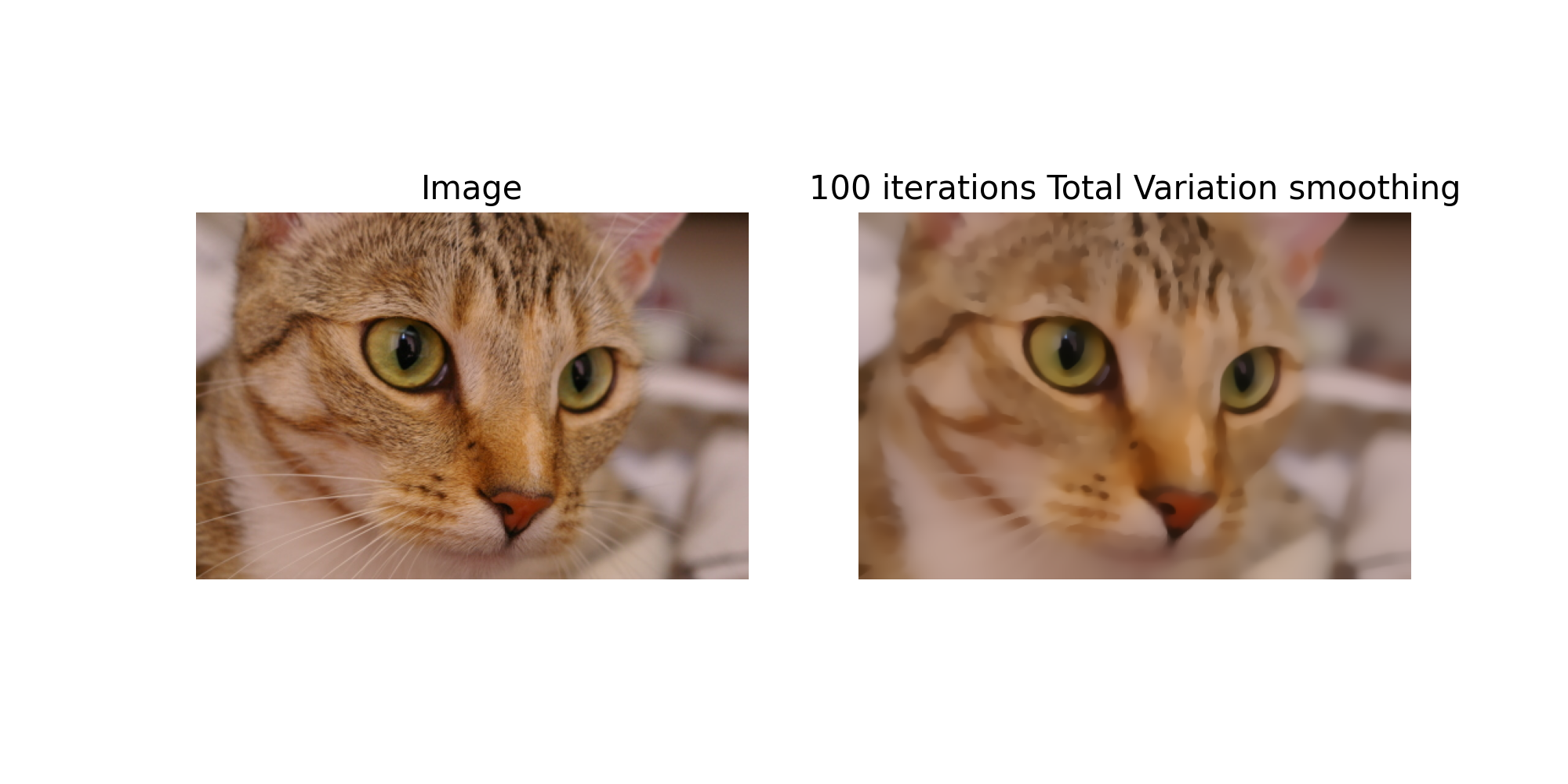
_DiffusionTotal variation (TV) diffusion operator, featuring an inhomogeneous isotropic diffusion tensor. It can be used for edge-enhancing smoothing. It reduces the diffusion intensity in locations characterised by large gradients, effectively achieving edge-preservation. The diffusion operator formulation of total variation regularization stems from the Euler-Lagrange equations associated to the problem of minimizing the TV regularization functional.
The gradient of the operator reads \(\nabla\phi(\mathbf{f})=-\mathrm{div}(\mathbf{D}(\mathbf{f})\boldsymbol{\nabla}\mathbf{f})\), deriving from the total variation potential \(\phi\). In the TV classical (untame) formulation, it holds \(\phi=\Vert \boldsymbol{\nabla}\mathbf{f}\Vert_{2,1}=\sum_{i=0}^{N_{tot}-1}\vert(\boldsymbol{\nabla}\mathbf{f})_i\vert\). A similar definition holds for its tame version (recommended).
The TV diffusion tensor is defined, for the \(i\)-th pixel, as:
\[\begin{split}\big(\mathbf{D}(\mathbf{f})\big)_i = (g(\mathbf{f}))_i \;\mathbf{I} = \begin{pmatrix}(g(\mathbf{f}))_i & 0\\ 0 & (g(\mathbf{f}))_i\end{pmatrix}.\end{split}\]The diffusivity can be defined in two possible ways:
in the tame case as
\[(g(\mathbf{f}))_i = \frac{\beta} { \sqrt{\beta^2+ \vert (\boldsymbol{\nabla} \mathbf{f})_i \vert ^2}}, \quad \forall i\]in the untame case as
\[(g(\mathbf{f}))_i = \frac{1} { \vert (\boldsymbol{\nabla} \mathbf{f})_i \vert}, \quad \forall i.\]The tame formulation amounts to an approximation of the TV functional very similar to the Huber loss approach. The parameter \(\beta\) controls the quality of the smooth approximation of the \(L^2\) norm \(\vert (\boldsymbol{\nabla} \mathbf{f})_i \vert\) involved in the TV approach. Lower values correspond to better approximations but typically lead to larger computational cost.
We recommended using the tame version; the untame one is unstable.
- Parameters:
dim_shape (
NDArrayShape) – Shape of the input array.beta (
Real) – Contrast parameter, determines the magnitude above which image gradients are preserved. Defaults to 1.tame (
bool) – Whether tame or untame version should be used. Defaults toTrue(tame, recommended).sampling (
Real,list[Real]) – Sampling step (i.e. distance between two consecutive elements of an array). Defaults to 1.
- Returns:
op – Total variation diffusion operator.
- Return type:
Example
import numpy as np
import matplotlib.pyplot as plt
import pyxu.opt.solver as pysol
import pyxu.abc.solver as pysolver
import pyxu.opt.stop as pystop
import pyxu_diffops.operator as pyxop
import skimage as skim

# Import RGB image
image = skim.data.cat().astype(float)
print(image.shape)  # (300, 451, 3)

# Move color-stacking axis to front (needed for pyxu stacking convention)
image = np.moveaxis(image, 2, 0)
print(image.shape)  # (3, 300, 451)

# Instantiate diffusion operator
tv_diffop = pyxop.TotalVariationDiffusion(dim_shape=(3, 300, 451), beta=2)

# Define PGD solver, with stopping criterion and starting point x0
stop_crit = pystop.MaxIter(n=100)

# Perform 50 gradient flow iterations starting from x0
PGD = pysol.PGD(f=tv_diffop, show_progress=False, verbosity=100)
PGD.fit(**dict(mode=pysolver.SolverMode.BLOCK, x0=image, stop_crit=stop_crit,
               tau=2/tv_diffop.diff_lipschitz))
tv_smoothed_image = PGD.solution()

# Reshape images for plotting.
image = np.moveaxis(image, 0, 2)
tv_smoothed_image = np.moveaxis(tv_smoothed_image, 0, 2)

# Plot
fig, ax = plt.subplots(1, 2, figsize=(10, 5))
ax[0].imshow(image.astype(int))
ax[0].set_title("Image", fontsize=15)
ax[0].axis('off')
ax[1].imshow(tv_smoothed_image.astype(int))
ax[1].set_title("100 iterations Total Variation smoothing", fontsize=15)
ax[1].axis('off')
(
Source code,png,hires.png,pdf)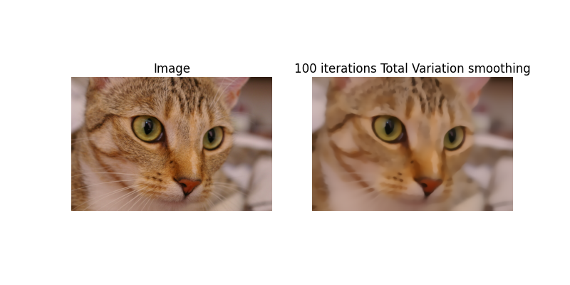
- class CurvaturePreservingDiffusionOp(dim_shape, curvature_preservation_field=None, sampling=1)[source]#
Bases:
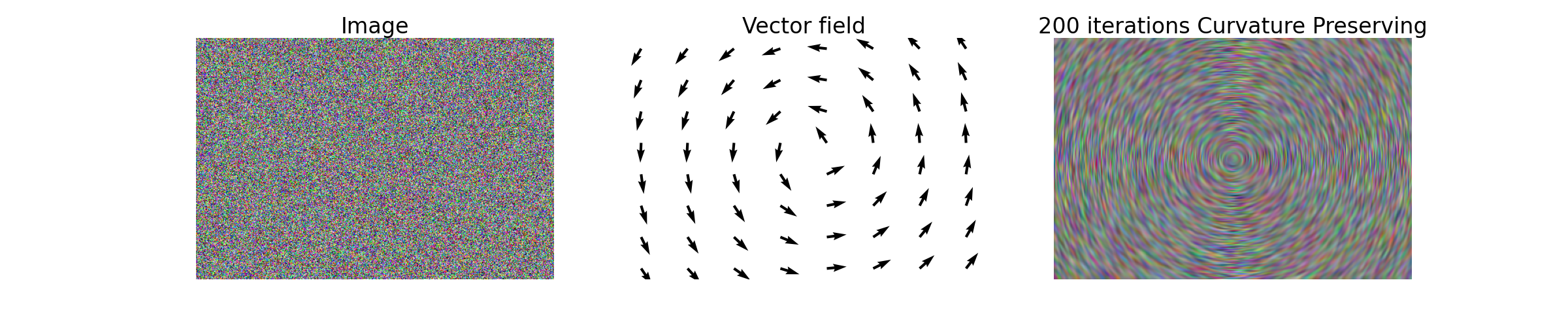
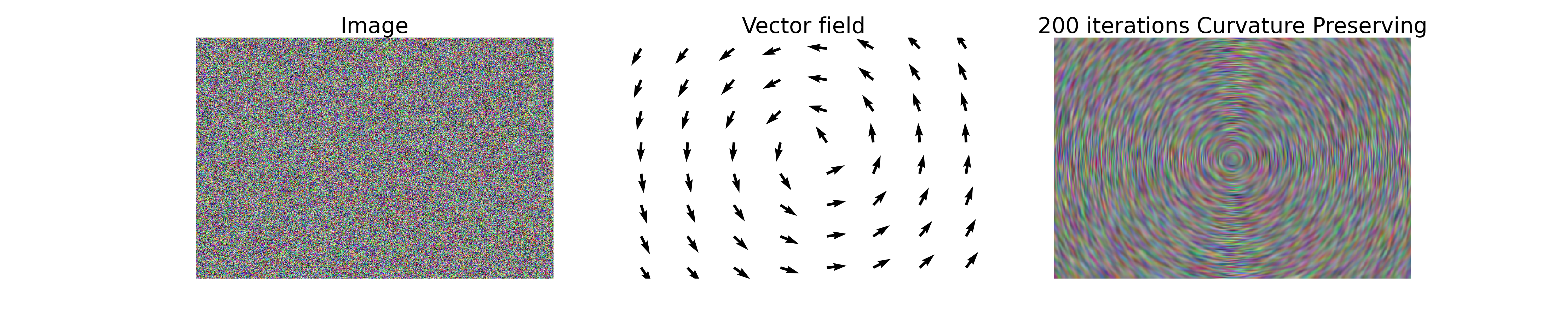
_DiffusionCurvature preserving diffusion operator [Tschumperle]. This trace-based operator promotes curvature preservation along a given vector field \(\mathbf{w}\), defined by a \(2\)-dimensional vector \(\mathbf{w}_i\in\mathbb{R}^2\) for each pixel \(i\).
The gradient of the operator reads
\[\frac{\partial\mathbf{f}}{\partial t} = -\mathrm{trace}\big(\mathbf{T}(\mathbf{w})\mathbf{H}(\mathbf{f})\big) - (\nabla\mathbf{f})^T \mathbf{J}_{\mathbf{w}}\mathbf{w},\]where the trace diffusion tensor \(\mathbf{T}(\mathbf{f})\) is defined, for the \(i\)-th pixel, as
\[\big(\mathbf{T}(\mathbf{f})\big)_i=\mathbf{w}_i\mathbf{w}_i^T.\]The curvature preserving diffusion operator does not admit a potential.
- Parameters:
- Returns:
op – Curvature preserving diffusion operator.
- Return type:
Example
import numpy as np
import matplotlib.pyplot as plt
import pyxu.operator.linop.diff as pydiff
import pyxu.opt.solver as pysol
import pyxu.abc.solver as pysolver
import pyxu.opt.stop as pystop
import pyxu_diffops.operator as pyxop
import skimage as skim

# Define random image
image = 255 * np.random.rand(3, 300, 451)

# Define vector field, diffusion process will preserve curvature along it
image_center = np.array(image.shape[1:]) / 2 + [0.25, 0.25]
curvature_preservation_field = np.zeros((2, np.prod(image.shape[1:])))
curv_pres_1 = np.zeros(image.shape[1:])
curv_pres_2 = np.zeros(image.shape[1:])
for i in range(image.shape[1]):
    for j in range(image.shape[2]):
        theta = np.arctan2(-i + image_center[0], j - image_center[1])
        curv_pres_1[i, j] = np.cos(theta)
        curv_pres_2[i, j] = np.sin(theta)
curvature_preservation_field[0, :] = curv_pres_1.reshape(1, -1)
curvature_preservation_field[1, :] = curv_pres_2.reshape(1, -1)
curvature_preservation_field = curvature_preservation_field.reshape(2, *image.shape[1:])

# Define curvature-preserving diffusion operator
CurvPresDiffusionOp = pyxop.CurvaturePreservingDiffusionOp(dim_shape=(3, 300, 451),
                                                            curvature_preservation_field=curvature_preservation_field)

# Perform 500 gradient flow iterations
stop_crit = pystop.MaxIter(n=200)
PGD_curve = pysol.PGD(f=CurvPresDiffusionOp, g=None, show_progress=False, verbosity=100)

PGD_curve.fit(**dict(mode=pysolver.SolverMode.BLOCK, x0=image, stop_crit=stop_crit, acceleration=False,
                     tau=1 / CurvPresDiffusionOp.diff_lipschitz))
curv_smooth_image = PGD_curve.solution()

# Reshape images for plotting.
image = np.moveaxis(image, 0, 2)
curv_smooth_image = np.moveaxis(curv_smooth_image, 0, 2)
# Rescale for better constrast
curv_smooth_image -= np.min(curv_smooth_image)
curv_smooth_image /= np.max(curv_smooth_image)
curv_smooth_image *= 255

# Plot
fig, ax = plt.subplots(1, 3, figsize=(30, 6))
ax[0].imshow(image.astype(int), cmap="gray", aspect="auto")
ax[0].set_title("Image", fontsize=30)
ax[0].axis('off')
ax[1].quiver(curv_pres_2[::40, ::60], curv_pres_1[::40, ::60])
ax[1].set_title("Vector field", fontsize=30)
ax[1].axis('off')
ax[2].imshow(curv_smooth_image.astype(int), cmap="gray", aspect="auto")
ax[2].set_title("200 iterations Curvature Preserving", fontsize=30)
ax[2].axis('off')
(
Source code,png,hires.png,pdf)
- class AnisEdgeEnhancingDiffusionOp(
- dim_shape,
- beta=1.0,
- m=4.0,
- sigma_gd_st=2,
- smooth_sigma_st=0,
- sampling=1,
- freezing_arr=None,
- matrix_based_impl=False,
- gpu=False,
- dtype=None,
Bases:
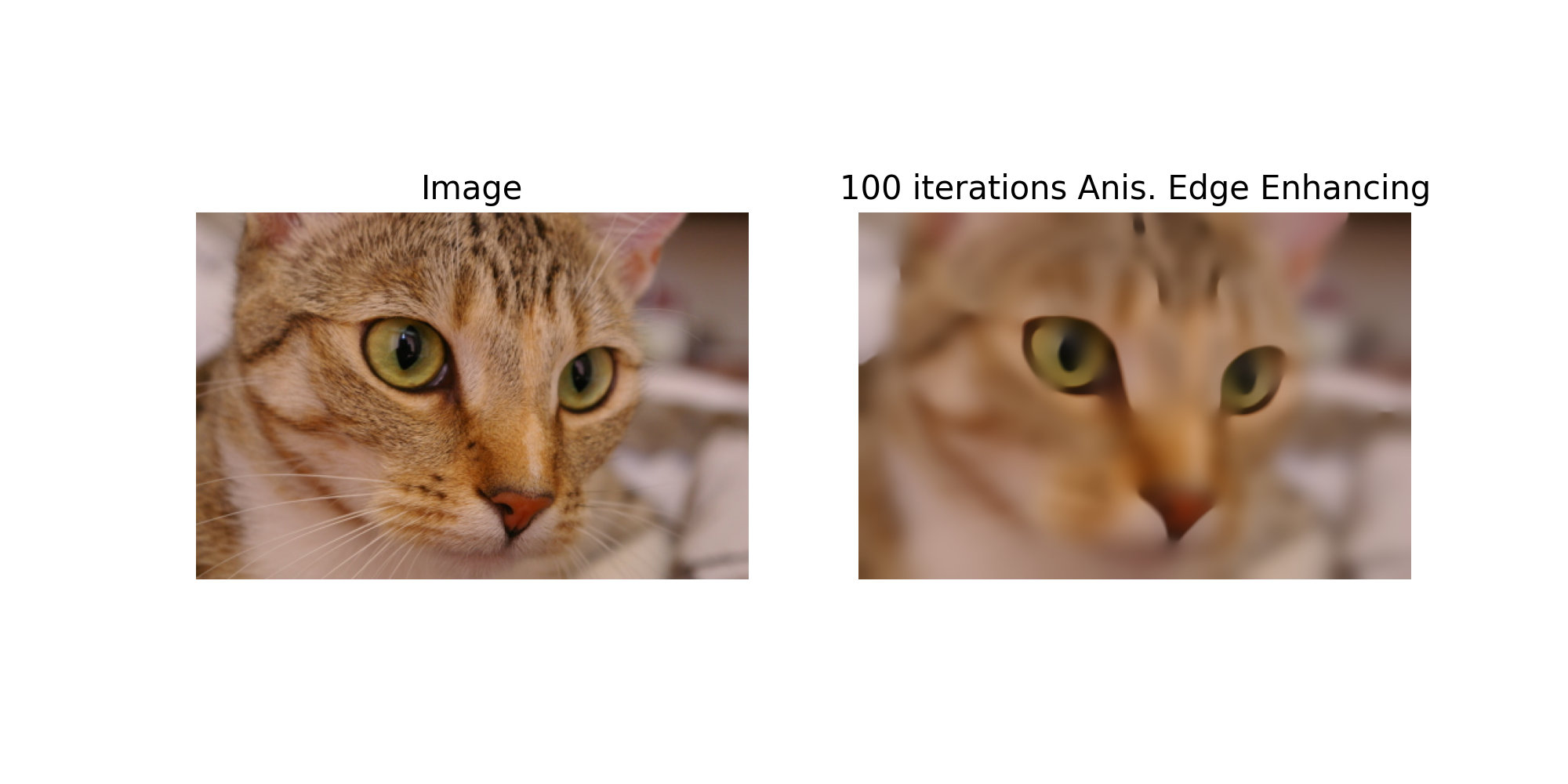
_DiffusionAnisotropic edge-enhancing diffusion operator, featuring an inhomogeneous anisotropic diffusion tensor defined as in [Weickert]. The diffusion tensor is defined as a function of the
StructureTensor, which is a tensor describing the properties of the image in the neighbourhood of each pixel. This diffusion operator allows edge enhancement by reducing the flux in the direction of the eigenvector of the structure tensor with largest eigenvalue. Essentially, smoothing across the detected edges is inhibited in a more sophisticated way compared to isotropic approaches, by considering not only the local gradient but its behaviour in a neighbourhood of the pixel.The gradient of the operator reads \(-\mathrm{div}(\mathbf{D}(\mathbf{f})\boldsymbol{\nabla}\mathbf{f})\).
Let \(\mathbf{v}_0^i,\mathbf{v}_1^i\) be the eigenvectors of the \(i\)-th pixel structure tensor \(S_i\), with eigenvalues \(e_0^i, e_1^i\) sorted in decreasing order. The diffusion tensor is defined, for the \(i\)-th pixel, as the symmetric positive definite tensor:
\[\big(\mathbf{D}(\mathbf{f})\big)_i = \lambda_0^i\mathbf{v}_0^i(\mathbf{v}_0^i)^T+\lambda_1^i\mathbf{v}_1^i(\mathbf{v}_1^i)^T,\]where the smoothing intensities along the two eigendirections are defined, to achieve edge-enhancing, as
\[\begin{split}\lambda_0^i &= g(e_0^i) := \begin{cases} 1 & \text{if } e_0^i = 0 \\ 1 - \exp\big(\frac{-C}{(e_0^i/\beta)^m}\big) & \text{if } e_0^i >0, \end{cases}\\ \lambda_1^i &= 1,\end{split}\]where \(\beta\) is a contrast parameter, \(m\) controls the decay rate of \(\lambda_0^i\) as a function of \(e_0^i\), and \(C\in\mathbb{R}\) is a normalization constant (see [Weickert]).
Since \(\lambda_1^i \geq \lambda_0^i\), the smoothing intensity is stronger in the direction of the second eigenvector of \(\mathbf{S}_i\), and therefore perpendicular to the (locally averaged) gradient. Moreover, \(\lambda_0^i\) is a decreasing function of \(e_0^i\), which indicates that when the gradient magnitude is high (sharp edges), smoothing in the direction of the gradient is inhibited, i.e., edges are preserved.
In general, the diffusion operator does not admit a potential. However, if the diffusion tensor is evaluated at some image \(\tilde{\mathbf{f}}\) and kept fixed to \(\mathbf{D}(\tilde{\mathbf{f}})\), the operator derives from the potential \(\Vert\sqrt{\mathbf{D}(\tilde{\mathbf{f}})}\boldsymbol{\nabla}\mathbf{f}\Vert_2^2\). By doing so, the smoothing directions and intensities are fixed according to the features of an image of interest. This can be achieved passing a freezing array at initialization. In such cases, a matrix-based implementation is recommended for efficiency.
- Parameters:
dim_shape (
NDArrayShape) – Shape of the input array.beta (
Real) – Contrast parameter, determines the gradient magnitude for edge enhancement. Defaults to 1.m (
Real) – Decay parameter, determines how quickly the smoothing effect changes as a function of \(e_0^i/\beta\). Defaults to 4.sigma_gd_st (
Real) – Gaussian width of the gaussian derivative involved in the structure tensor computation. Defaults to 2.smooth_sigma_st (
Real) – Width of the Gaussian filter smoothing the structure tensor (local averaging). Defaults to 0 (recommended).sampling (
Real,list[Real]) – Sampling step (i.e. distance between two consecutive elements of an array). Defaults to 1.freezing_arr (
NDArray) – Array at which the diffusion tensor is evaluated and then frozen.matrix_based_impl (
bool) – Whether to use matrix based implementation or not. Defaults to False. Recommended to setTrueif afreezing_arris passed.gpu (bool)
dtype (dtype[Any] | None | type[Any] | _SupportsDType[dtype[Any]] | str | tuple[Any, int] | tuple[Any, SupportsIndex | Sequence[SupportsIndex]] | list[Any] | _DTypeDict | tuple[Any, Any])
- Returns:
op – Anisotropic edge-enhancing diffusion operator.
- Return type:
Example
import numpy as np
import matplotlib.pyplot as plt
import pyxu.opt.solver as pysol
import pyxu.abc.solver as pysolver
import pyxu.opt.stop as pystop
import pyxu_diffops.operator as pyxop
import skimage as skim

# Import RGB image
image = skim.data.cat().astype(float)
print(image.shape)  # (300, 451, 3)

# Move color-stacking axis to front (needed for pyxu stacking convention)
image = np.moveaxis(image, 2, 0)
print(image.shape)  # (3, 300, 451)

# Instantiate diffusion operator
edge_enh_diffop = pyxop.AnisEdgeEnhancingDiffusionOp(dim_shape=(3, 300, 451), beta=10)

# Define PGD solver, with stopping criterion and starting point x0
stop_crit = pystop.MaxIter(n=100)

# Perform 50 gradient flow iterations starting from x0
PGD = pysol.PGD(f=edge_enh_diffop, show_progress=False, verbosity=100)
PGD.fit(**dict(mode=pysolver.SolverMode.BLOCK, x0=image, stop_crit=stop_crit,
               tau=2 / edge_enh_diffop.diff_lipschitz))
edge_enh_image = PGD.solution()

# Reshape images for plotting.
image = np.moveaxis(image, 0, 2)
edge_enh_image = np.moveaxis(edge_enh_image, 0, 2)

# Plot
fig, ax = plt.subplots(1, 2, figsize=(10, 5))
ax[0].imshow(image.astype(int))
ax[0].set_title("Image", fontsize=15)
ax[0].axis('off')
ax[1].imshow(edge_enh_image.astype(int))
ax[1].set_title("100 iterations Anis. Edge Enhancing", fontsize=15)
ax[1].axis('off')
(
Source code,png,hires.png,pdf)
- class AnisCoherenceEnhancingDiffusionOp(
- dim_shape,
- alpha=0.1,
- m=1,
- sigma_gd_st=2,
- smooth_sigma_st=4,
- sampling=1,
- diff_method_struct_tens='gd',
- freezing_arr=None,
- matrix_based_impl=False,
- gpu=False,
- dtype=None,
Bases:
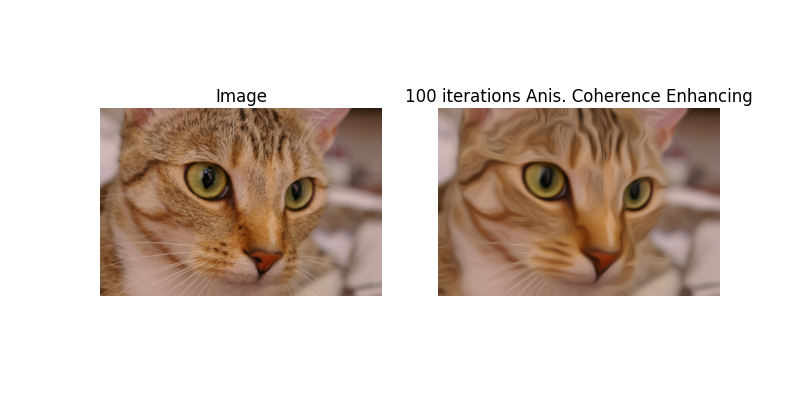
_DiffusionAnisotropic coherence-enhancing diffusion operator, featuring an inhomogeneous anisotropic diffusion tensor defined as in [Weickert]. The diffusion tensor is defined as a function of the
StructureTensor, which is a tensor describing the properties of the image in the neighbourhood of each pixel. This diffusion operator allows coherence enhancement by increasing the flux in the direction of the eigenvector of the structure tensor with smallest eigenvalue, with an intensity which depends on the image coherence, which is measured as \((e_0-e_1)^2\). Stronger coherence leads to stronger smoothing.The gradient of the operator reads \(-\mathrm{div}(\mathbf{D}(\mathbf{f})\boldsymbol{\nabla}\mathbf{f})\).
Let \(\mathbf{v}_0^i,\mathbf{v}_1^i\) be the eigenvectors of the \(i\)-th pixel structure tensor \(S_i\), with eigenvalues \(e_0^i, e_1^i\) sorted in decreasing order. The diffusion tensor is defined, for the \(i\)-th pixel, as the symmetric positive definite tensor:
\[\big(\mathbf{D}(\mathbf{f})\big)_i = \lambda_0^i\mathbf{v}_0^i(\mathbf{v}_0^i)^T+\lambda_1^i\mathbf{v}_1^i(\mathbf{v}_1^i)^T,\]where the smoothing intensities along the two eigendirections are defined, to achieve coherence-enhancing, as
\[\begin{split}\lambda_0^i &= \alpha,\\ \lambda_1^i &= h(e_0^i, e_1^i) := \begin{cases} \alpha & \text{if } e_0^i=e_1^i \\ \alpha + (1-\alpha) \exp \big(\frac{-C}{(e_0^i-e_1^i)^{2m}}\big) & \text{otherwise}, \end{cases}\end{split}\]where \(\alpha \in (0, 1)\) controls the smoothing intensity along the first eigendirection, \(m\) controls the decay rate of \(\lambda_0^i\) as a function of \((e_0^i-e_1^i)\), and \(C\in\mathbb{R}\) is a constant.
For regions with low coherence, smoothing is performed uniformly along all directions with intensity \(\lambda_1^i \approx \lambda_0^i = \alpha\). For regions with high coherence, we have \(\lambda_1^i \approx 1 > \lambda_0^i = \alpha\), hence the smoothing intensity is higher in the direction orthogonal to the (locally averaged) gradient.
In general, the diffusion operator does not admit a potential. However, if the diffusion tensor is evaluated at some image \(\tilde{\mathbf{f}}\) and kept fixed to \(\mathbf{D}(\tilde{\mathbf{f}})\), the operator derives from the potential \(\Vert\sqrt{\mathbf{D}(\tilde{\mathbf{f}})}\boldsymbol{\nabla}\mathbf{f}\Vert_2^2\). By doing so, the smoothing directions and intensities are fixed according to the features of an image of interest. This can be achieved passing a freezing array at initialization. In such cases, a matrix-based implementation is recommended for efficiency.
- Parameters:
dim_shape (
NDArrayShape) – Shape of the input array.alpha (
Real) – Anisotropic parameter, determining intensity of smoothing inhibition along the (locally averaged) image gradient. Defaults to 1e-1.m (
Real) – Decay parameter, determines how quickly the smoothing effect changes as a function of \(e_0^i/\beta\). Defaults to 1.sigma_gd_st (
Real) – Gaussian width of the gaussian derivative involved in the structure tensor computation (ifdiff_method_struct_tens="gd"). Defaults to 2.smooth_sigma_st (
Real) – Width of the Gaussian filter smoothing the structure tensor (local averaging). Defaults to 4.sampling (
Real,list[Real]) – Sampling step (i.e. distance between two consecutive elements of an array). Defaults to 1.diff_method_struct_tens (
str) – Differentiation method for structure tensor computation. Must be either ‘gd’ or ‘fd’. Defaults to ‘gd’.freezing_arr (
NDArray) – Array at which the diffusion tensor is evaluated and then frozen.matrix_based_impl (
bool) – Whether to use matrix based implementation or not. Defaults to False. Recommended to setTrueif afreezing_arris passed.gpu (bool)
dtype (dtype[Any] | None | type[Any] | _SupportsDType[dtype[Any]] | str | tuple[Any, int] | tuple[Any, SupportsIndex | Sequence[SupportsIndex]] | list[Any] | _DTypeDict | tuple[Any, Any])
- Returns:
op – Anisotropic coherence-enhancing diffusion operator.
- Return type:
Example
import numpy as np
import matplotlib.pyplot as plt
import pyxu.opt.solver as pysol
import pyxu.abc.solver as pysolver
import pyxu.opt.stop as pystop
import pyxu_diffops.operator as pyxop
import skimage as skim

# Import RGB image
image = skim.data.cat().astype(float)
print(image.shape)  # (300, 451, 3)

# Move color-stacking axis to front (needed for pyxu stacking convention)
image = np.moveaxis(image, 2, 0)
print(image.shape)  # (3, 300, 451)

# Instantiate diffusion operator
coh_enh_diffop = pyxop.AnisCoherenceEnhancingDiffusionOp(dim_shape=(3, 300, 451), alpha=1e-3)

# Define PGD solver, with stopping criterion and starting point x0
stop_crit = pystop.MaxIter(n=100)

# Perform 50 gradient flow iterations starting from x0
PGD = pysol.PGD(f=coh_enh_diffop, show_progress=False, verbosity=100)
PGD.fit(**dict(mode=pysolver.SolverMode.BLOCK, x0=image, stop_crit=stop_crit,
               tau=2 / coh_enh_diffop.diff_lipschitz))
coh_enh_image = PGD.solution()

# Reshape images for plotting.
image = np.moveaxis(image, 0, 2)
coh_enh_image = np.moveaxis(coh_enh_image, 0, 2)

# Plot
fig, ax = plt.subplots(1, 2, figsize=(10, 5))
ax[0].imshow(image.astype(int))
ax[0].set_title("Image", fontsize=15)
ax[0].axis('off')
ax[1].imshow(coh_enh_image.astype(int))
ax[1].set_title("100 iterations Anis. Coherence Enhancing", fontsize=15)
ax[1].axis('off')
(
Source code,png,hires.png,pdf)
- class AnisDiffusionOp(
- dim_shape,
- alpha=0.1,
- sigma_gd_st=1,
- sampling=1,
- diff_method_struct_tens='fd',
- freezing_arr=None,
- matrix_based_impl=False,
- gpu=False,
- dtype=None,
Bases:
_DiffusionAnisotropic diffusion operator, featuring an inhomogeneous anisotropic diffusion tensor. The diffusion tensor is defined as a function of the
StructureTensor, which is a tensor describing the properties of the image in the neighbourhood of each pixel. This diffusion operator allows anisotropic smoothing by reducing the flux in the direction of the eigenvector of the structure tensor with largest eigenvalue. Essentially, the (locally averaged) gradient is preserved.The gradient of the operator reads \(-\mathrm{div}(\mathbf{D}(\mathbf{f})\boldsymbol{\nabla}\mathbf{f})\).
Let \(\mathbf{v}_0^i,\mathbf{v}_1^i\) be the eigenvectors of the \(i\)-th pixel structure tensor \(S_i\), with eigenvalues \(e_0^i, e_1^i\) sorted in decreasing order. The diffusion tensor is defined, for the \(i\)-th pixel, as the symmetric positive definite tensor:
\[\big(\mathbf{D}(\mathbf{f})\big)_i = \lambda_0^i\mathbf{v}_0^i(\mathbf{v}_0^i)^T+\lambda_1^i\mathbf{v}_1^i(\mathbf{v}_1^i)^T,\]where the smoothing intensities along the two eigendirections are defined, to achieve anisotropic smoothing, as
\[\begin{split}\lambda_0^i &= \alpha,\\ \lambda_1^i &= 1,\end{split}\]where \(\alpha \in (0, 1)\) controls the smoothing intensity along the first eigendirection.
In general, the diffusion operator does not admit a potential. However, if the diffusion tensor is evaluated at some image \(\tilde{\mathbf{f}}\) and kept fixed to \(\mathbf{D}(\tilde{\mathbf{f}})\), the operator derives from the potential \(\Vert\sqrt{\mathbf{D}(\tilde{\mathbf{f}})}\boldsymbol{\nabla}\mathbf{f}\Vert_2^2\). By doing so, the smoothing directions and intensities are fixed according to the features of an image of interest. This can be achieved passing a freezing array at initialization. In such cases, a matrix-based implementation is recommended for efficiency.
- Parameters:
dim_shape (
NDArrayShape) – Shape of the input array.alpha (
Real) – Anisotropic parameter, determining intensity of smoothing inhibition along the (locally averaged) image gradient. Defaults to 1e-1.sigma_gd_st (
Real) – Gaussian width of the gaussian derivative involved in the structure tensor computation (ifdiff_method_struct_tens="gd"). Defaults to 1.smooth_sigma_st (
Real) – Width of the Gaussian filter smoothing the structure tensor (local averaging). Defaults to 1.sampling (
Real,list[Real]) – Sampling step (i.e. distance between two consecutive elements of an array). Defaults to 1.diff_method_struct_tens (
str) – Differentiation method for structure tensor computation. Must be either ‘gd’ or ‘fd’. Defaults ot ‘fd’.freezing_arr (
NDArray) – Array at which the diffusion tensor is evaluated and then frozen.matrix_based_impl (
bool) – Whether to use matrix based implementation or not. Defaults to False. Recommended to setTrueif afreezing_arris passed.gpu (bool)
dtype (dtype[Any] | None | type[Any] | _SupportsDType[dtype[Any]] | str | tuple[Any, int] | tuple[Any, SupportsIndex | Sequence[SupportsIndex]] | list[Any] | _DTypeDict | tuple[Any, Any])
- Returns:
op – Anisotropic diffusion operator.
- Return type: